Performance Estimation#
When integrating the RadarImager into a production line, one important question is usually: How long does it take until an image is available on the client?
Answering this precisely is difficult because the total latency depends on many factors, including the installation geometry, trigger position, object speed, image dimensions, number of selected layers, and the computational load caused by the chosen parameter set.
This chapter explains a practical step-by-step estimation approach. It assumes that the conveyor or object speed is known. For this reason, some values are described as distances and others as times, because they can be converted easily:
time = distance / speeddistance = speed × time
Interactive estimator available
Use the dedicated Performance Estimation Tool when you want a full-width live calculator to do the estimation for you.
Estimate, not guaranteed value
The formulas in this chapter and the Performance Estimation Tool are intended for practical estimation. Actual values can differ depending on the exact installation, parameter set, network configuration, and the performance of the receiving client.
Estimation strategy#
The total delay until the image is available on the client can be divided into three parts:
- Data acquisition distance
- Processing time
- Transmission time
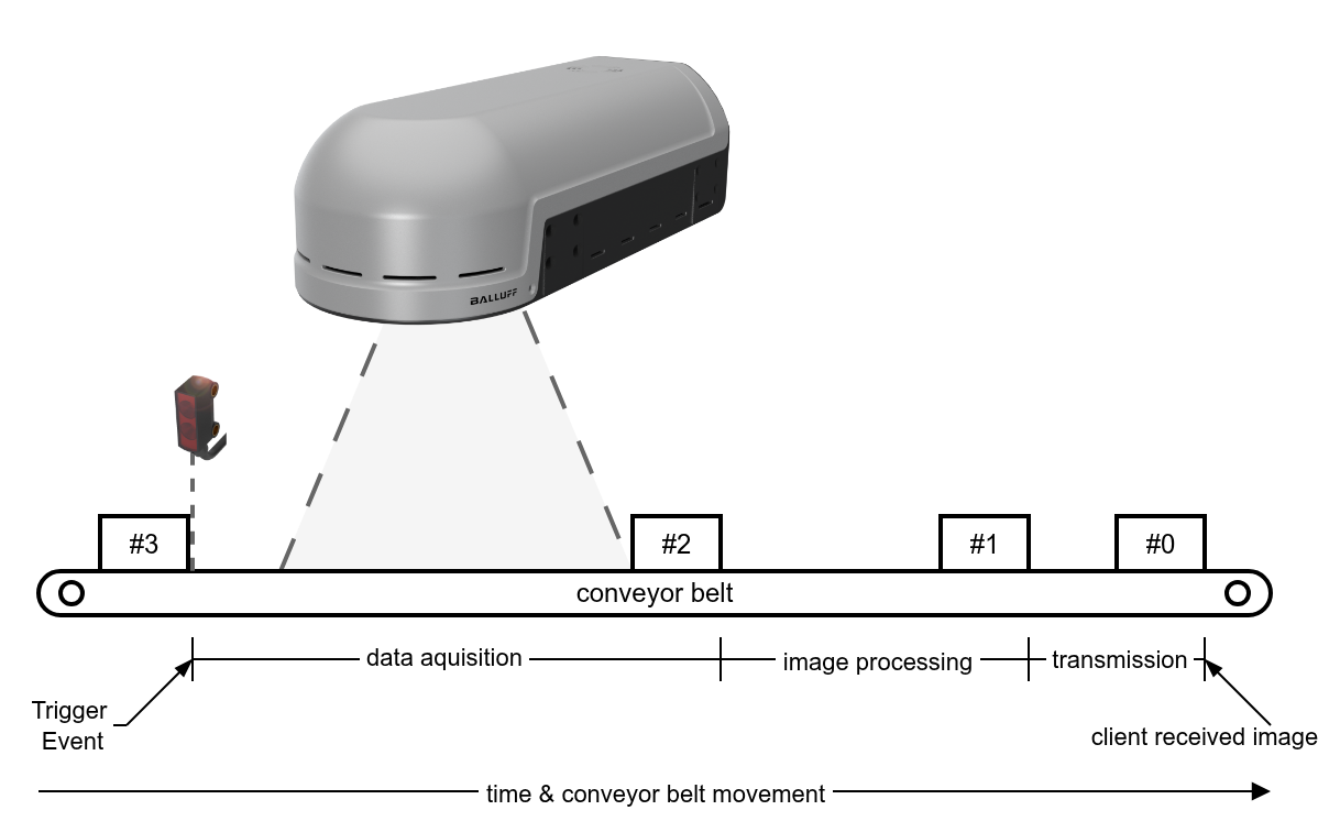
This can be written as:
totalTime ≈ acquisitionTime + processingTime + transmissionTime
1. Data acquisition distance#
Before image processing can begin, the object must move completely through the relevant acquisition area. This section estimates the distance required to acquire all data needed for image generation.
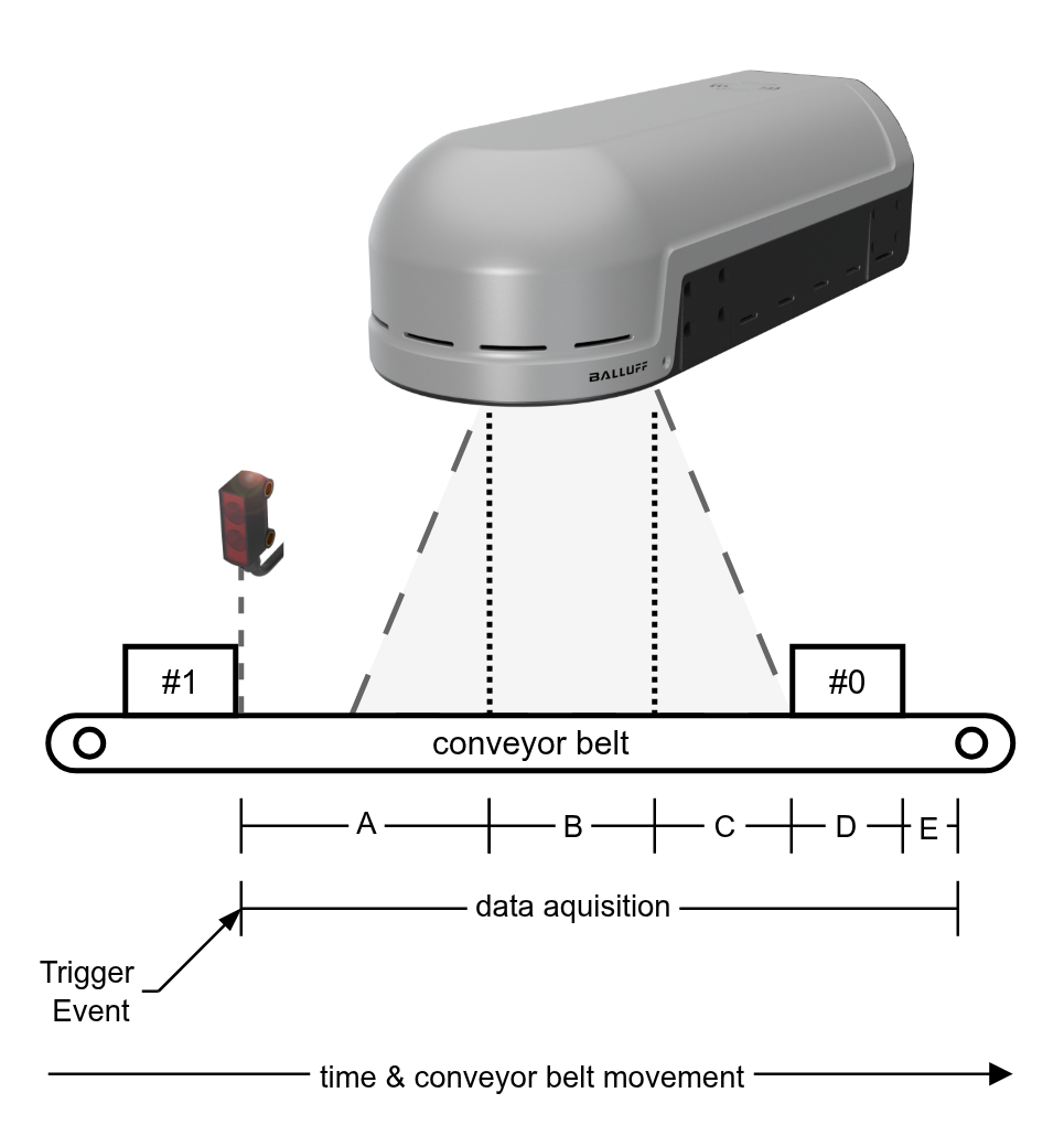
Symbolic trigger position in the figure
The position of the trigger sensor in the figure is only symbolic. Measured from the system reference line,
the trigger sensor on Port1 can be mounted anywhere from 0 mm up to just below objectLengthX,
configured via offsetDistanceX.
If the trigger sensor is mounted directly at the system reference line (offsetDistanceX = 0 mm),
the RadarImager can still use measurement data recorded before the trigger event to cover the angular acquisition range.
For practical mounting rules, see Hardware installation.
[A] Trigger offset: offsetDistanceX#
The first contribution is the distance between the trigger sensor and the RadarImager system reference line.
This distance is configured with offsetDistanceX
and depends on the mounting position of the trigger sensor.
[B] Active radar area#
The object must fully pass the active radar area of the RadarImager. For practical estimation, this active area can be approximated as:
70 mm
[C] Additional distance caused by angular coverage#
The antennas do not only radiate vertically downward. Depending on the deepest processed layer, the object must travel an additional distance until all required data has been recorded.
This additional distance can be approximated as:
additionalDistance ≈ min(distanceZToDeepestLayerOfInterest × 3 / √3, 100 mm)
where distanceZToDeepestLayerOfInterest
is given in mm.
Depth dependency
The deeper the processed volume is configured, the larger this additional distance becomes.
For practical use, this term is limited to a maximum of 100 mm.
If possible, mount the RadarImager so that the layers of interest are as close as possible to the minimum selectable distance of 100 mm.
[D] Configured image length: objectLengthX#
The configured object length objectLengthX
also contributes directly.
The RadarImager must wait until the recorded object has completely passed the relevant radar area
before image processing can start.
[E] Acquisition tolerance#
For practical estimation, an additional fixed reserve should be included to cover the small tolerance between the ideal geometric image position and the exact point at which all required measurement data is available for image generation.
This reserve can be approximated as:
32 mm
Approximate acquisition distance#
The resulting distance before image processing can begin can therefore be estimated as:
acquisitionDistance ≈ [A] offsetDistanceX +
                      [B] 70 mm +
                      [C] min(distanceZToDeepestLayerOfInterest × 3 / √3, 100 mm) +
                      [D] objectLengthX +
                      [E] 33 mm
2. Processing time#
After data acquisition is complete, the RadarImager starts processing the image. Estimating this processing time precisely with a general formula is difficult, because it depends on many parameters and on their interaction.
The most relevant influences are usually:
objectLengthXdistanceZToDeepestLayerOfInterest- the number of selected layers in
layerSelection.indexes - special parameter combinations that increase the computational load, which is not always predictable
Vision parameters and normalization
For production environments, all vision parameters should normally remain at their default settings and
are not recommended to be changed. The normalization kind is set to normAbsKind PREDEFINED.
The Performance Estimation Tool assumes the system is configured accordingly.
The following parameter does not influence the system performance significantly:
No universal closed-form formula
A precise project-independent formula for processingTime is currently not available.
It can be estimated with the Performance Estimation Tool.
If exact values are required, please contact Support
for a project-specific performance estimation.
Assumption used by the estimation tool
The Performance Estimation Tool provides an estimate and assumes that the minimum distance between two object edges is large enough that one image processing cycle can finish before the next one must be processed. If this condition is not met parallel processing might occur wich can increase the overall time significantly.
Practical measurement on a real system#
Once a real setup is available, the best reference is the transmitted metadata field TimestampDuration
from the GenDC container.
TimestampDuration measures the time from the trigger event until the start of image data transmission.
It therefore already includes:
- the trigger offset travel
- the acquisition distance through the radar area
- the internal image processing time
This means that the processing time can be estimated on a real installation as:
processingTime[s] ≈ TimestampDuration[µs] / 1,000,000 - acquisitionTime[s]
as long as acquisitionTime is estimated from the real geometry and the configured objectSpeedX.
For background on the metadata fields, see Image-to-Object Mapping.
3. Transmission time#
The transmission time from the RadarImager to the client can be estimated from the amount of transferred data and the Gigabit Ethernet link speed.
The transferred data volume depends mainly on:
objectLengthX- the number of selected layers in
layerSelection.indexes - whether
upscaleImageis enabled
The distance of pixels in the xy plane is approximately 1.03 mm.
With an image height of 256 pixels and 3 color channels,
the payload can be estimated as:
payloadBytes ≈ (objectLengthX[m] / 0.00103 m) × 256 × 3 × nLayers + 40
This includes a total of 40 Bytes metadata transmitted with the GenDC container.
The transmission time is then approximately:
transmissionTime[s] ≈ payloadBytes × 8 / 1,000,000,000
For a 1 Gbit/s link (1,000,000,000 bit/s) this becomes:
transmissionTime[s] ≈ totalTransmittedBytes × 8 / 1,000,000,000
Using the pixel-distance approximation above and including the fixed 40 B metadata, the practical rule of thumb remains usable for quick estimates, but strictly speaking the small fixed overhead slightly increases the transmission time per image. The estimator tool adds the 40 B automatically to the payload calculation.
where nLayers is the number of selected layers in layerSelection.indexes.
Effect of upscaleImage
If upscaleImage is enabled,
the image width and height are both doubled.
This increases the transmitted data volume by approximately a factor of 4.
In production environments, upscaleImage should normally remain disabled.
What is not included
This estimate does not fully model protocol overhead, buffering, switch behavior, host-side packet processing, client-side decoding, or application-side image handling.
Practical recommendation#
For an initial project estimate:
- Determine the installation geometry and set a realistic
offsetDistanceX. - Determine the planned
objectLengthX. - Determine the required depth using
distanceZToDeepestLayerOfInterest. - Count the selected layers in
layerSelection.indexes. - Keep
upscaleImagedisabled for production estimates. - Estimate the transmission time with the simplified formula above.
- Once hardware is available, validate the real internal latency with
TimestampDuration.
If you already know your intended installation, the minimum spacing between objects, the expected object frequency,
and the main parameters such as objectLengthX and nLayers, Balluff support can provide a more precise performance estimate.